Getting Started¶

This guide will help you install and start using the Siglent Report Generator.

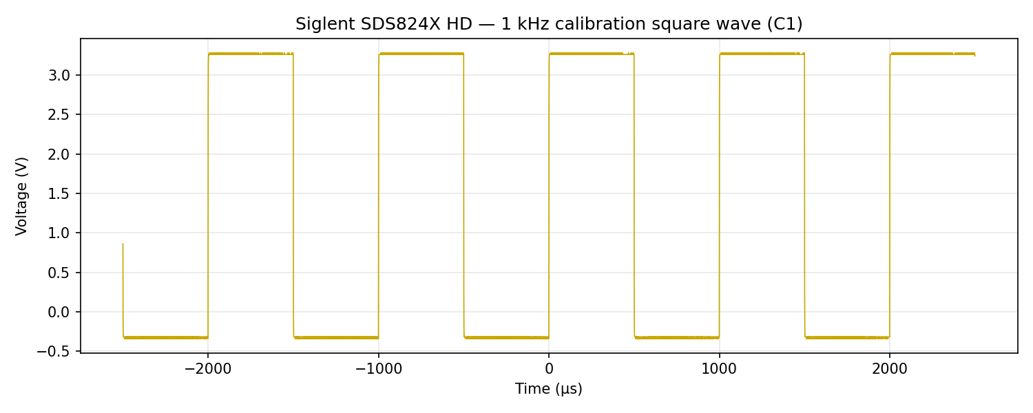
The generator turns real captures into analysed reports. Here is the kind of input it works from — a genuine 1 kHz calibration square wave captured from a Siglent SDS824X HD:

Installation¶

Option 1: Install from Source (Development)¶

If you have the source code:

# Navigate to the project directory
cd SCPI-Instrument-Control

# Install with report generator dependencies
pip install -e ".[report-generator]"

Option 2: Install from PyPI¶

pip install "SCPI-Instrument-Control[report-generator]"

Verify Installation¶

# Check that the command is available
siglent-report-generator --version

# Or try launching it
siglent-report-generator

Dependencies¶

The Report Generator requires:

Required:
PyQt6 - GUI framework
matplotlib - Plotting
numpy - Numerical computing
scipy - Signal processing
Pillow - Image handling
Optional:
reportlab - PDF generation (highly recommended)
requests - LLM API calls (for AI features)
h5py - HDF5 file support

All dependencies are installed automatically with pip install -e ".[report-generator]".

Launching the Application¶

GUI Application¶

# Method 1: Using the installed command
siglent-report-generator

# Method 2: Using Python module
python -m scpi_control.report_generator.app

Standalone Executable¶

If you have a pre-built executable:

Windows:

# Navigate to the executable folder
cd dist/SiglentReportGenerator

# Run it
SiglentReportGenerator.exe

Linux:

# Navigate to the executable folder
cd dist/SiglentReportGenerator

# Run it
./SiglentReportGenerator

GUI Overview¶

Main Window Layout¶

The Report Generator window is divided into two main sections:

┌─────────────────────────────────────────────────────────┐
│  File  Settings  Help                                   │
├──────────────────────────┬──────────────────────────────┤
│                          │                              │
│  DATA IMPORT             │  AI ASSISTANT                │
│                          │                              │
│  ┌────────────────────┐  │  Status: Connected           │
│  │ Imported Waveforms │  │                              │
│  │                    │  │  Chat History...             │
│  │ • CH1 - file1.npz  │  │                              │
│  │ • CH2 - file1.npz  │  │                              │
│  └────────────────────┘  │                              │
│                          │                              │
│  [Import Waveforms...]   │  [Type question...]          │
│  [Import Images...]      │                              │
│  [Clear All]             │  [Generate Summary]          │
│                          │  [Analyze Waveforms]         │
│  REPORT METADATA         │  [Interpret Measurements]    │
│                          │                              │
│  Title: ____________     │                              │
│  Technician: _______     │                              │
│  Date: ______________    │                              │
│  Equipment: _________    │                              │
│  ...                     │                              │
│                          │                              │
│  [Generate PDF Report]   │                              │
│  [Generate MD Report]    │                              │
│                          │                              │
└──────────────────────────┴──────────────────────────────┘

Left Panel - Data & Configuration¶

Data Import Section:

Shows list of imported waveforms
Buttons to import waveforms and images
Clear all data button

Report Metadata:

Scrollable form with all metadata fields
Required: Title, Technician, Test Date
Optional: Equipment details, environmental conditions, branding

Generation Buttons:

Generate PDF Report
Generate Markdown Report

Right Panel - AI Assistant¶

Status Display:

Shows LLM connection status
Displays current model

Chat Interface:

Type questions about your data
View AI responses
Clear chat history

Quick Actions:

Generate Summary - Auto-create executive summary
Analyze Waveforms - Get signal quality insights
Interpret Measurements - Explain pass/fail results

Creating Your First Report¶

Step 1: Prepare Sample Data¶

First, let's create some sample waveform data:

# Run the example script to generate sample data
python examples/report_generation_example.py

This creates sample waveform files in example_reports/ directory.

Or, if you have existing oscilloscope data, use that!

Step 2: Import Waveforms¶

Launch the application

siglent-report-generator

Click "Import Waveforms..."
Select your waveform files
Supported formats: .npz, .csv, .mat, .h5, .hdf5
You can select multiple files at once
The waveforms will appear in the list
Verify the import
Each channel should appear as a separate item
Format: ChannelName - filename.ext

Step 3: Fill in Metadata¶

Scroll through the metadata form and fill in the fields:

Required Fields:

Report Title - e.g., "Power Supply Ripple Test"
Technician - Your name
Test Date - Defaults to current date/time

Optional but Recommended:

Equipment Model - e.g., "SDS2104X Plus"
Equipment ID - Serial number
Test Procedure - Reference number
Project Name - What project this belongs to
Customer - If applicable
Notes - Any additional context

Environmental Conditions:

Temperature
Humidity
Location

Branding (Optional):

Company Name
Company Logo (click "Select Logo...")
Header/Footer Text

Step 4: Generate Your Report¶

Choose format:
Click "Generate PDF Report" for PDF
Click "Generate Markdown Report" for Markdown
Choose save location:
A file dialog will appear
Select where to save the report
Use a descriptive filename
Wait for generation:
A progress dialog appears
Report generation typically takes 5-30 seconds
Depends on number of waveforms and plots
Success!
A confirmation dialog shows the save location
Open the report to view it

Step 5: Review Your Report¶

PDF Report Sections:

Header - Company logo and name (if configured)
Title - Report title centered
Metadata Table - All test information
Overall Result - PASS/FAIL status
Sections:
Test Setup
Waveform Captures (with plots)
Measurements (with tables)
FFT Analysis (if included)
Footer - Generation date and company name

Markdown Report:

Same content as PDF
Markdown-formatted for version control
Plots saved in plots/ subdirectory
Can be converted to other formats

Working with Images¶

Importing Images¶

Click "Import Images..."
Select image files:
Supported formats: .png, .jpg, .jpeg, .bmp
Multiple selection supported
Images are stored for inclusion in reports

Image Use Cases¶

Setup Photos - Show physical test configuration
Screenshots - Capture oscilloscope screen
Diagrams - Include circuit diagrams or schematics
Reference Images - Compare with expected waveforms

Annotating Plots¶

Waveform, region-zoom, FFT and comparison-overlay plots can carry your own markup on top of the automatic capture data: text labels, vertical and horizontal reference lines, and shaded spans. Waveform, FFT and comparison-overlay plots can also carry a figure caption beneath the plot; a region zoom cannot — it is a sub-view of its parent waveform's already-captioned figure, so it inherits the parent's annotations (clipped to the region's time window) but has no caption of its own.

Annotating a report plot

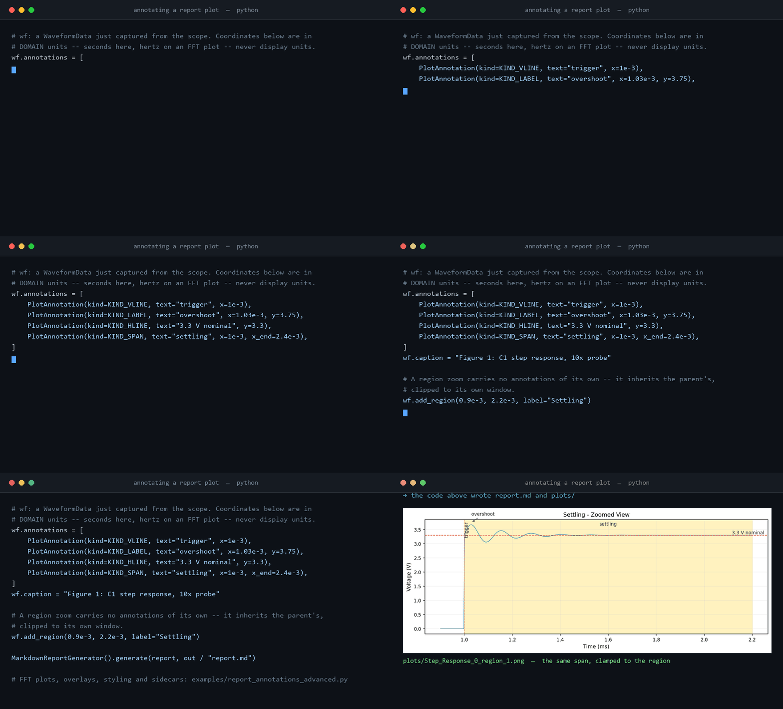
The four kinds:

Label — a text callout pinned to an (x, y) point, with an arrow, for calling out a specific feature (an edge, a glitch, a measurement point).
Vertical line — a dashed line at a given x, for marking a moment in time (a trigger point, an edge).
Horizontal line — a dashed line at a given y, for marking a threshold or nominal level (a spec limit, a rail voltage).
Span — a shaded band between two x values, for marking a window (a settling region, a glitch duration).

Coordinates are always in domain units — seconds on a time-domain plot (waveform, region, comparison), hertz on an FFT plot — never the display units a given plot happens to use (a waveform plot may show microseconds, a region plot milliseconds, an FFT plot megahertz). The renderer converts domain units to display units when it draws the plot, so an annotation's position does not shift if a plot's display scale changes.

GUI route¶

Select a waveform in the imported list.
Click Annotate….
Pick an anchor from the dropdown (waveform start/end/midpoint, max, min, or a region's start, midpoint or end) to prefill coordinates, or enter them by hand.
Enter the annotation text, choose the kind, and click Add.
Repeat for as many annotations as you need, and set a figure caption if you want one.
Click Save to file to write the annotations to the sidecar (see below).

API route¶

Annotations are plain PlotAnnotation objects assigned to a WaveformData's annotations list (or a TestSection's fft_annotations for an FFT plot). Two runnable examples:

examples/report_annotations.py — all four kinds plus a caption on one waveform plot, rendered to a PDF. Start here.
examples/report_annotations_advanced.py — every surface beyond that: all four plot types, per-annotation overrides against PlotStyle defaults, a region zoom inheriting clipped annotations, the sidecar save/restore round-trip, and the anchor list the Annotate... dialog offers.

The image above is generated by scripts/media/make_annotation_gif.py, which executes the code it renders — regenerate it after changing the annotation API.

Persistence¶

Saving writes a <source>.annotations.json sidecar next to the waveform's source file, keyed by channel. A save merges by channel: it reads whatever sidecar already exists and only replaces the channels you saved, so saving one channel of a multi-channel capture does not erase the other channels' annotations, and saving a waveform's annotations without touching its FFT data leaves that channel's previously saved FFT annotations intact. Re-importing the source file restores the saved annotations and caption automatically; loading is idempotent, so importing the same file twice does not duplicate them.

Limitations¶

Comparison/batch overlay annotations are API-only and do not persist. An overlay spans several source files, so there is no single sidecar that could own it — set them in Python for each report you generate.
FFT plot annotations have no GUI route for creating or saving them. They can be set from Python via save_annotations(waveforms, fft={...}). Restoring them on re-import requires the caller to set the TestSection's fft_channel to the channel they were saved under; the app does not currently do this itself, so today automatic restore only happens for an API caller who sets fft_channel explicitly. The Annotate… dialog edits waveform annotations only.
Overlapping labels are not auto-spaced. If two labels land on top of each other, nudge one with text_dx/text_dy (offsets from the anchor, as a fraction of the axis span) rather than expecting automatic layout.
Label offsets are not clamped to the plot area. text_dx/text_dy are applied as-is, and matplotlib does not grow the axes to fit annotation text, so an offset that lands outside the data range puts the text outside the plot box — a large positive text_dy on a label near the top of the trace typically collides with the plot title. Only the label kind takes offsets at all: vertical-line and span text is pinned just inside the top of the axes, and horizontal-line text to the right edge at its own line's height, so those stay within the plot box. Keep label offsets small (the 0.06 default is roughly the right scale) and check the rendered plot rather than assuming a big offset will be reined in.
A literal * or _ in a caption can corrupt the surrounding emphasis markup, in both PDF and Markdown reports. Both formats deliberately interpret *text* and _text_ in a caption as emphasis — the Markdown generator emits captions unescaped, and the PDF generator's markdown-to-ReportLab conversion pairs */_ into <i> tags — so this is a real feature, not a bug, when the pairing is intentional. An unpaired literal * or _ breaks that pairing and corrupts the rendered text either way. Avoid a lone * or _ in captions unless you mean it as emphasis.

New Report (Ctrl+N) - Clear all data and start fresh
Exit (Ctrl+Q) - Close the application

LLM Configuration... - Configure AI features
Opens the LLM settings dialog
See LLM Setup for details

About - Information about the application
Shows version
Lists features
Links to documentation

Keyboard Shortcuts¶

Ctrl+N - New report
Ctrl+Q - Quit application
Enter (in chat) - Send chat message

Common Tasks¶

Creating Multiple Reports from Same Data¶

Import waveforms once
Fill in metadata
Generate first report (e.g., PDF)
Change title or notes as needed
Generate second report (e.g., Markdown)

Batch Processing¶

For batch processing multiple tests:

Use the Programmatic API
Write a Python script to:
Load multiple waveform sets
Apply templates
Generate all reports
See examples/report_generation_example.py for reference

Saving Time with Templates¶

Instead of re-entering metadata every time:

Create a report with your standard settings
Save it as a template (API feature)
Load the template for each new test
See Template Guide for details

Troubleshooting¶

"reportlab not installed" error¶

PDF generation requires reportlab:

pip install reportlab

"Failed to load waveform" error¶

Check file format:

Supported: NPZ, CSV, MAT, HDF5
Unsupported: Binary scope formats

Verify file structure:

Must contain time and voltage data
See API Reference for expected format

Application won't start¶

Check dependencies:

pip install -e ".[report-generator]"

Check PyQt6 platform plugins:

# Windows
set QT_QPA_PLATFORM_PLUGIN_PATH=<python>/Lib/site-packages/PyQt6/Qt6/plugins

# Linux
export QT_QPA_PLATFORM_PLUGIN_PATH=<python>/lib/python3.x/site-packages/PyQt6/Qt6/plugins

Generation is slow¶

Normal for:

Large waveforms (millions of samples)
Many channels
Complex plots

Speed tips:

Use Markdown for faster generation
Reduce plot resolution
Limit waveform length if possible

Out of memory errors¶

Reduce memory usage:

Process waveforms one at a time
Use lower resolution plots
Close other applications

Next Steps¶

Now that you have the basics:

Enable AI Features → - Set up Ollama for AI analysis
Use Templates → - Save time with reusable configurations
Learn the API → - Automate report generation

Getting Help¶

Documentation - You're reading it!
Examples - See examples/report_generation_example.py
Issues - Report bugs on GitHub
Discussions - Ask questions on GitHub Discussions